SCTP (New Protocol within TCP/IP)

INTRODUCTION

SCTP is a reliable transport protocol operating over IP. SCTP is more akin to TCP than UDP, however it yields additional features to TCP while still supporting much of the same functionality. So SCTP is connection oriented and implements the same congestion/flow control. Detection of data corruption, loss of data and duplication of data is achieved by using checksums and sequence numbers. A selective retransmission mechanism is applied to correct loss or corruption of data.

In the TCP/IP network model, SCTP resides in the transport layer, alongside TCP and UDP. The transport layer handles communication among programs in a network. This involves accepting data from the application layer, and repackaging it (perhaps fragmenting the data) so it may be passed on to the network layer. In addition the transport layer will also ensure the data arrives correctly on the other end. A transport protocol in essence is a set of rules that govern how data is sent between communicating nodes.

The network layer is used for; basic communication, addressing and routing, IP is usually used. The application layer consists of end-user applications and the link layer defines network hardware and device drivers.


Comparing SCTP to TCP

SCTP and TCP have some distinct differences, yet also many similarities. In this section we will explore their similarities and then discuss the major ways in which they differ.

Similarities

Startup: to establish an association between two nodes, both protocols will exchange a series of messages. There are differences in the way these messages are exchanged and their format, but they hold the same purpose- to set up an end-to-end connection (association or connection).

Reliability and Ordering: both SCTP and TCP implement mechanisms to endure the successful delivery of user datagrams. This includes reliable and ordered data delivery.

Congestion Control: this is a critical element in any transport protocol. It regulates the flow of data entering the network, limiting it to accommodate for occurrences of congestion. SCTP and TCP hold the same congestion control mechanism- Additive Increase, Multiplicative Decrease (AIMD) congestion window management.

Closing Down: both protocols have two different close procedures, a graceful close and an abortive one. The graceful close will ensure that all user data in the queue will be delivered before the association is terminated. The abortive close occurs during errors.

Differences

There are two key differences between TCP and SCTP:

· Multihoming

· Multistreaming

These are new features in SCTP and are what really set the two protocols apart.

Multihoming: an essential property of SCTP is its support of multi-homed nodes, i.e. nodes which can be reached under several IP addresses. If we allow SCTP nodes to support more than one IP address, during network failure data can be rerouted to alternative destination IP addresses. This makes the nodes more tolerant against physical network failures and other problems of that kind.

Multistreaming: is an effective way to limit Head-of-Line Blocking. The benefit in having multiple independent data streams is if a packet is lost in one stream, while that stream blocks to wait for the retransmission the remaining unaffected streams can continue to send data. In TCP if a packet is lost, the connection effectively grinds to a halt while it waits for the retransmission to be sent.


An SCTP association is equivalent to a TCP connection, they both represent an end-to-end relationship between two transmitting nodes.

Multistreaming can be achieved in TCP, however it involves opening multiple TCP connections which each act as a stream to send data. This differs from multistreaming in SCTP where all the streams reside in a single association. Opening multiple TCP connections is TCP-unfriendly, which means that a pair of communicating nodes will obtain a larger proportion of the available channel bandwidth. Thus, SCTP is more TCP-friendly in this regard.

Although multihoming and multistreaming may be where SCTP and TCP differ most, the two protocols exhibit other differences, which are also important to discuss.

Security at Startup: SCTP and TCP both carry out an exchange of messages to establish an end-to-end relationship. The way these messages are sent however, are different. Traditional TCP uses a three-way handshake, whereas SCTP uses a four-way handshake. A signed state cookie is involved in the SCTP four-way handshake, which helps to protect from denial of service attacks.

A denial of service attack is where resources are tied up on the server side so that it is impossible to respond to legitimate connections. The attacker issues vast amounts of SYN requests (a message requesting set-up of a connection) to the server and when it receives the SYN, ACK it simply discards it, not bothering to respond with an ACK. This causes the server to retain the partial state that was allocated after the SYN request, and if carried out repetitively will lead to a denial of service.

SCTP protects against denial of service attacks with the use of a cookie. The cookie is bundled with the INIT-ACK from the server to the client. The server does not record the association or keep a transmission control block (TCB), rather it derives the TCB from the cookie, which is sent back from the client inside the COOKIE-ECHO. Since it has no knowledge of the association till the client responds with a COOKIE-ECHO, it becomes resilient to denial of service attacks.

There may at first appear to be an overhead to sending four messages, however user data can be bundled in the last two SCTP packets.

Data Delivery: Data transmission in TCP is byte-stream oriented; in SCTP, it is message-oriented. In TCP, data is transported as a consecutive stream of bytes between two endpoints, so user message boundaries are not preserved when they are on the wire between two end points. Parts of one message may be sent with parts of another message, in a single data packet. This means that some kind of message-delineation is required by the application, to inform the receiver, the message length and the amount to read. The receiving application will need to do some complex buffering and framing to reconstruct the messages.

SCTP, in contrast, makes an explicit demarcation of user message boundaries. Each message is delivered as a complete read, which lifts a lot of the work off the application layer. An exception to this is when the message is larger than the maximum packet size. Although, parts of two user messages will never be put into a single data packet.

Unordered Delivery: SCTP allows for data to be sent reliably but unordered. This has benefits when dealing with large amounts of independent transactions, e.g. components in a web page. TCP has no such facility.

SACKs: All acknowledgements in SCTP are with SACKs. They are useful as they indicate if there are any gaps in the transmission, i.e. missing blocks. TCP does not make explicit use of SACKs but can be configured to support them. However, TCP can only report four missing data packets in a SACK, SCTP allows for much larger amounts to be reported.

Closing Association: Despite the fact that both TCP and SCTP have graceful close mechanisms, there is a slight difference in what these mechanisms permit. TCP allows what is known as the “half-closed” state, where one endpoint stays open while the other endpoint closes. SCTP does not allow this, both endpoints must close when the shutdown primitive is issued. One reason for not putting the half-closed state in SCTP was the lack of use of it: very few applications require it.

Strict Aliasing

What is strict aliasing?
Strict aliasing is an assumption, made by the C (or C++) compiler, that dereferencing pointers to objects of different types will never refer to the same memory location (i.e. alias eachother.)

Examples

Pointers to different built in types do not alias:

0int16_t* foo;
1int32_t* bar;

The compiler will assume that *foo and *bar never refer to the same location.
Pointers to aggregate or union types with differing tags do not alias:

0typedef struct
1{
2 uint16_t a;
3 uint16_t b;
4 uint16_t c;
5} Foo;
6
7typedef struct
8{
9 uint16_t a;
10 uint16_t b;
11 uint16_t c;
12} Bar;
13
14Foo* foo;
15Bar* bar;

The compiler will assume that *foo and *bar never refer to the same location, even though the contents of the structures are the same.

Pointers to aggregate or union types which differ only by name may alias:

0typedef struct
1{
2 uint16_t a;
3 uint16_t b;
4 uint16_t c;
5} Foo;
6
7typedef Foo Bar;
8
9Foo* foo;
10Bar* bar;

The compiler will assume that *foo and *bar may refer to the same location, and will not perform the optimizations decribed below.

Benefits to The Strict Aliasing Rule
When the compiler cannot assume that two object are not aliased, it must act very conservatively when accessing memory. For example:

0typedef struct
1{
2 uint16_t a;
3 uint16_t b;
4 uint16_t c;
5} Sample;
6
7void
8test( uint32_t* values,
9 Sample* uniform,
10 uint64_t count )
11{
12 uint64_t i;
13
14 for (i=0;i 15 {
16 values[i] += (uint32_t)uniform->b;
17 }
18}

Compiled with -fno-strict-aliasing -O3 -std=c99 on the 64 bit build of GNU C version 3.4.1 (CELL 2.3, Jul 21 2005) (powerpc64-linux) for the Cell PPU.

0test:
1 li 10, 0 # i = 0
2 cmpld 7, 10, 5 # done = (i==count)
3 bgelr- 7 # if (done) return
4 mtctr 5 # ctr = count
5.L8:
6 sldi 11, 10, 2 # offset = i * 4
7 lwz 9, 4(4) # b = *(uniform+4)
8 addi 10, 10, 1 # i++
9 lwzx 5, 11, 3 # value = *(values+offset)
10 add 0, 5, 9 # value = value + b
11 stwx 0, 11, 3 # *(values+offset) = value
12 bdnz .L8 # if (ctr--) goto .L8
13 blr # return

In this case uniform->b must be loaded during each iteration of the loop. This is because the compiler cannot be certain that values does not overlap b in memory. If, in fact, they do overlap, the programmer would expect that uniform->b would be properly updated and the values stored into the values array adjusted accordingly. The only method for the compiler to guarantee these results is reloading uniform->b at every iteration.

It was noted that this case is extremely uncommon in most code and the decision was made to presume objects of different types are not aliased and to be more aggresive with optimizations. It is certain the fact this presumption would break some existing code was discussed in detail. It must have been decided that those most likely to use memory aliasing techniques for optimization are are few and those that do use it are the most willing and capable of making the necessary changes.

The result, even for this small case, can make a significant performance impact. Compiled with -fstrict-aliasing -Wstrict-aliasing=2 -O3 -std=c99 on the 64 bit build of GNU C version 3.4.1 (CELL 2.3, Jul 21 2005) (powerpc64-linux) for the Cell PPU.

0test:
1 li 11,0 # i = 0
2 cmpld 7,11,5 # done = (i == count)
3 bgelr- 7 # if (done) return
4 lhz 4,2(4) # b = uniform.b
5 mtctr 5 # ctr = count
6.L8:
7 sldi 9,11,2 # offset = i * 4
8 addi 11,11,1 # i++
9 lwzx 5,9,3 # value = *(values+offset)
10 add 0,5,4 # value = value + b
11 stwx 0,9,3 # *(values+offset) = value
12 bdnz .L8 # if (ctr--) goto .L8
13 blr # return

The load of b is now only done once, outside the loop. For more examples of optimizations for non-aliasing memory see: Demystifying The Restrict Keyword
Casting Compatible Types
Aliases are permitted for types that only differ by qualifier or sign.

0uint32_t
1test( uint32_t a )
2{
3 uint32_t* const a0 = &a;
4 uint32_t* volatile a1 = &a;
5 int32_t* a2 = (int32_t*)&a;
6 int32_t* const a3 = (int32_t*)&a;
7 int32_t* volatile a4 = (int32_t*)&a;
8 const int32_t* const a5 = (int32_t*)&a;
9
10 (*a0)++;
11 (*a1)++;
12 (*a2)++;
13 (*a3)++;
14 (*a4)++;
15
16 return (*a5);
17}

In this case a0-a5 are all valid aliases of a and this function will return (a + 5).
GCC has two flags to enable warnings related to strict aliasing. -Wstrict-aliasing enables warnings for most common errors related to type-punning. -Wstrict-aliasing=2 attempts to warn about a larger class of cases, however false positives may be returned.
Casting through a union (1)
The most commonly accepted method of converting one type of object to another is by using a union type as in this example:

0typedef union
1{
2 uint32_t u32;
3 uint16_t u16[2];
4}
5U32;
6
7uint32_t
8swap_words( uint32_t arg )
9{
10 U32 in;
11 uint16_t lo;
12 uint16_t hi;
13
14 in.u32 = arg;
15 hi = in.u16[0];
16 lo = in.u16[1];
17 in.u16[0] = lo;
18 in.u16[1] = hi;
19
20 return (in.u32);
21}

This method is not properly called casting at all (although it may be called type-punning) as the value is simplied copied into a union which permits aliasing among its members. From a performance point of view, this method relies on the ability of the optimizer to remove the redundant stores and loads. When using recent versions of GCC, if the transformation is reasonably simple, it is very likely that the compiler will be able to remove the redundancies and produce an optimal code sequence.
Strictly speaking, reading a member of a union different from the one written to is undefined in ANSI/ISO C99 except in the special case of type-punning to a char*, similar to the example below: Casting to char*. However, it is an extremely common idiom and is well-supported by all major compilers. As a practical matter, reading and writing to any member of a union, in any order, is acceptable practice.
For example, when compiled with GNU C version 4.0.0 (Apple Computer, Inc. build 5026) (powerpc-apple-darwin8), the argument is simply rotated 16 bits.

0swap_words:
1 rlwinm r3,r3,16,0xffffffff
2 blr

When compiled with -fstrict-aliasing -O3 -Wstrict-aliasing -std=c99 on GNU C version 3.4.1 (CELL 2.3, Jul 21 2005) (powerpc64-linux) for the Cell PPU, the loads and stores are removed but the instruction sequence is less than optimal.

0swap_words:
1 slwi 4,3,16 ; hi = arg << 16
2 rldicl 3,3,48,48 ; lo = arg >> 16
3 or 0,4,3 ; out = hi | lo;
4 rldicl 3,0,0,32 ; final = out & 0xffffffff
5 blr


In order to generate reasonably good code across both the GCC3 and GCC4 families, use C99 style intializers:

0uint32_t
1swap_words( uint32_t arg )
2{
3 U32 in = { .u32=arg };
4 U32 out = { .u16[0]=in.u16[1],
5 .u16[1]=in.u16[0] };
6
7 return (out.u32);
8}

Compiled with -fstrict-aliasing -O3 -Wstrict-aliasing -std=c99 on the 32 bit build of GNU C version 3.4.1 (CELL 2.3, Jul 21 2005) (powerpc64-linux) for the Cell PPU.

0swap_words:
1 stwu 1,-16(1) ; Push stack
2 rlwinm 3,3,16,0xffffffff ; Rotate 16 bits
3 addi 1,1,16 ; Pop stack
4 blr

It is a parculiarity of the 32 bit build of GCC 3.4.1 for the Cell PPU that the stack is always pushed and popped regardless of whether or not it is used.
This method is most valuable for use with primitive types which can be returned by value. This is because it relies on doing a complete copy of the object (by value) and removing the redundancies. With more complex aggregate or union types copying may be done on the stack or through the memcpy function and redundancies are harder to eliminate.
Casting through a union (2)
Casting proper may be done between a pointer to a type and a pointer to an aggregate or union type which contains a member of a compatible type, as in the following example:

0uint32_t
1swap_words( uint32_t arg )
2{
3 U32* in = (U32*)&arg;
4 uint16_t lo = in->u16[0];
5 uint16_t hi = in->u16[1];
6
7 in->u16[0] = hi;
8 in->u16[1] = lo;
9
10 return (in->u32);
11}

in is a pointer to a U32 type, which contains the member u32 which is of type uint32_t which is compatible with arg, which is also of type uint32_t.
The above source when compiled with GCC 4.0 with the -Wstrict-aliasing=2 flag enabled will generate a warning. This warning is an example of a false positive. This type of cast is allowed and will generate the appropriate code (see below). It is documented clearly that -Wstrict-aliasing=2 may return false positives.
Compiled with -fstrict-aliasing -O3 -Wstrict-aliasing -std=c99 on GNU C version 4.0.0 (Apple Computer, Inc. build 5026) (powerpc-apple-darwin8),

0swap_words:
1 stw r3,24(r1) ; Store arg
2 lhz r0,24(r1) ; Load hi
3 lhz r2,26(r1) ; Load lo
4 sth r0,26(r1) ; Store result[1] = hi
5 sth r2,24(r1) ; Store result[0] = lo
6 lwz r3,24(r1) ; Load result
7 blr ; Return

GCC is extremely poor at combining loads and stores done through a pointer to a union type as can be seen from the generated code above. The output is a very naive interpretation of the source and would perform badly compared to the previous examples on most architectures.

However, once this fact is accounted for, this method can be very useful. Rather than copying the argument by value, which is problematic on large or complex structures, a pointer can be passed in and the value modified directly. If the loads and stores can be combined in the source the results will usually be excellent.
"But when the address of a variable is taken, doesn't the compiler force it to be stored in memory rather than in a register?"

Yes, both a store and a load may then generated as part of the trace. However, when alias analysis is done it can be determined that the object cannot be changed another mechanism so the load and store may be marked as redundant and removed.
Do not rely on the compiler to combine loads and stores. The programmer is always better equipted to make those decisions based on alignment concerns and complex instruction penalty rules.

0uint16_t*
1swap_words( uint16_t* arg )
2{
3 U32* combined = (U32*)arg;
4 uint32_t start = combined->u32;
5 uint32_t lo = start >> 16;
6 uint32_t hi = start << 16;
7 uint32_t final = lo | hi;
8
9 combined->u32 = final;
10}

Compiled with -fstrict-aliasing -O3 -Wstrict-aliasing -std=c99 on GNU C version 4.0.0 (Apple Computer, Inc. build 5026) (powerpc-apple-darwin8),

0swap_words:
1 lwz r0,0(r3) ; Load arg
2 rlwinm r0,r0,16,0xffffffff ; Rotate 16 bits
3 stw r0,0(r3) ; Store arg
4 blr ; Return

If the above source is called as a non-inline function, there will be a signficant penalty on most architectures waiting for the load before the rotate and the store on return.
If the above source is called as a inline function, it can be safely assumed the load and store will be removed by the compiler as redundant.
In C99, a static inline function, which may be included in a header file, differs from automatic inlining in that the function may be defined multiple times (e.g. included by multiple source files). Each definition of a static inline function must be identical.

0static inline void
1swap_words( uint16_t* arg )
2{
3 U32* combined = (U32*)arg;
4 uint32_t start = combined->u32;
5 uint32_t lo = start >> 16;
6 uint32_t hi = start << 16;
7 uint32_t final = lo | hi;
8
9 combined->u32 = final;
10}

With some care, this method is the most appropriate for modifying large or complex structures by multiple types.
Casting through a union (3)
Occasionally a programmer may encounter the following INVALID method for creating an alias with a pointer of a different type:

0typedef union
1{
2 uint16_t* sp;
3 uint32_t* wp;
4} U32P;
5
6uint32_t
7swap_words( uint32_t arg )
8{
9 U32P in = { .wp = &arg };
10 const uint16_t hi = in.sp[0];
11 const uint16_t lo = in.sp[1];
12
13 in.sp[0] = lo;
14 in.sp[1] = hi;
15
16 return ( arg ); <-- RESULT IS UNDEFINED
17}

The problem with this method is although U32P does in fact say that sp is an alias for wp, it does not say anything about the relationship between the values pointed to by sp and wp. This differs in a critical way from "Casting Through a Union (1)" and "Casting Through a Union (2)" which both define aliases for the values being pointed to, not the pointers themselves.

The presumption of strict aliasing remains true: Two pointers of different types are assumed, except in a few very limited conditions specified in the C99 standard, not to alias. This is not one of those exceptions.
The above source when compiled with GCC 3.4.1 or GCC 4.0 with the -Wstrict-aliasing=2 flag enabled will NOT generate a warning. This should serve as an example to always check the generated code. Warnings are often helpful hints, but they are by no means exaustive and do not always detect when a programmer makes an error. Like any peice of software, a compiler has limits. Knowing them can only be helpful.
For example, when compiled with -fstrict-aliasing -O3 -Wstrict-aliasing -std=c99 on GNU C version 4.0.0 (Apple Computer, Inc. build 5026) (powerpc-apple-darwin8),

0swap_words: ; RETURNS ARG UNCHANGED
1 lhz r0,24(r1) ; Load lo from stack (What value?!)
2 lhz r2,26(r1) ; Load hi from stack (What value?!)
3 stw r3,24(r1) ; Store arg to stack
4 sth r0,26(r1) ; Store hi to stack
5 sth r2,24(r1) ; Store lo to stack
6 blr ; Return

In this case notice that because hi, lo and arg are assumed not to alias, the resulting order of instruction has no value:

* [Line 1]: lo is loaded from the stack before anything is stored to the stack
* [Line 2]: hi is loaded from the stack before anything is stored to the stack
* [Line 3]: arg is stored to the stack, but this value will not be read.
* [Line 4]: hi is stored to the stack, but this value will not be read.
* [Line 5]: lo is stored to the stack, but this value will not be read.

Or when compiled with -fstrict-aliasing -O3 -Wstrict-aliasing -std=c99 on the 64 bit build of GNU C version 3.4.1 (CELL 2.3, Jul 21 2005) (powerpc64-linux) for the Cell PPU.

0swap_words: # RETURNS ARG UNCHANGED
1 stw 3,48(1) # Store arg to stack
2 lhz 9,48(1) # Load hi
3 lhz 0,50(1) # Load lo
4 lwz 3,48(1) # Load arg
5 sth 0,48(1) # Store hi to stack
6 sth 9,50(1) # Store lo to stack
7 blr # Return

Or when compiled with -fstrict-aliasing -O3 -Wstrict-aliasing -std=c99 on the 32 bit build of GNU C version 3.4.1 (CELL 2.3, Jul 21 2005) (powerpc64-linux) for the Cell PPU.

0swap_words: # RETURNS ARG UNCHANGED
1 stwu 1,-16(1) # Push stack
2 addi 1,1,16 # Pop stack
3 blr # Return

Casting to char*
It is always presumed that a char* may refer to an alias of any object. It is therefore quite safe, if perhaps a bit unoptimal (for architecture with wide loads and stores) to cast any pointer of any type to a char* type.

0uint32_t
1swap_words( uint32_t arg )
2{
3 char* const cp = (char*)&arg;
4 const char c0 = cp[0];
5 const char c1 = cp[1];
6 const char c2 = cp[2];
7 const char c3 = cp[3];
8
9 cp[0] = c2;
10 cp[1] = c3;
11 cp[2] = c0;
12 cp[3] = c1;
13
14 return (arg);
15}

The converse is not true. Casting a char* to a pointer of any type other than a char* and dereferencing it is usually in volation of the strict aliasing rule.
In other words, casting from a pointer of one type to pointer of an unrelated type through a char* is undefined.

0uint32_t
1test( uint32_t arg )
2{
3 char* const cp = (char*)&arg;
4 uint16_t* const sp = (uint16_t*)cp;
5
6 sp[0] = 0x0001;
7 sp[1] = 0x0002;
8
9 return (arg);
10}

When compiled with -fstrict-aliasing -O3 -Wstrict-aliasing -std=c99 on the 64 bit build of GNU C version 3.4.1 (CELL 2.3, Jul 21 2005) (powerpc64-linux) for the Cell PPU.

0test:
1 stw 3, 48(1) # arg stored to stack
2 li 0, 1 # hi = 0x0001
3 li 9, 2 # lo = 0x0002
4 lwz 3, 48(1) # result = loaded from stack
5 sth 0, 48(1) # store hi to stack
6 sth 9, 50(1) # store lo to stack
7 blr # return (result) <-- RETURNS ARG UNCHANGED

As clarified by Pinskia, it is not deferencing a char* per se that is specifically recognized as a potential alias of any object, but any address referring to a char object. This includes an array of char objects, as in the following example which will also break the strict aliasing assumption.

0 char const cp[4] = { arg0, arg1, arg2, arg3 };
1 uint16_t* const sp = (uint16_t*)cp;
2
3 sp[0] = 0x0001;
4 sp[1] = 0x0002;

GCC RULE BREAKING
GCC allows type-punned values to be deferenced at independent locations in memory (i.e. different objects) when the source of the lvalue is not directly known.

0void
1set_value( uint64_t* c,
2 uint32_t a_val,
3 uint16_t b_val )
4{
5 uint32_t* a = (uint32_t*)c;
6 uint16_t* b = (uint16_t*)c;
7
8 a[0] = a_val; // <--- Address of c + 0
9 b[2] = b_val; // <--- Address of c + 4
10 b[3] = b_val; // <--- Address of c + 6
11}

When compiled with -fstrict-aliasing -O3 -Wstrict-aliasing -std=c99 on the 64 bit build of GNU C version 3.4.1 (CELL 2.3, Jul 21 2005) (powerpc64-linux) for the Cell PPU.

0set_value:
1 stw 4,0(3) # (c+0) = a_val
2 sth 5,6(3) # (c+6) = b_val
3 sth 5,4(3) # (c+4) = b_val
4 blr # return (c)

Note any use of c[0] here would be (more?) undefined because it would alias the uses of a and b.

0void
1set_value( uint64_t* c,
2 uint32_t a_val,
3 uint16_t b_val )
4{
5 uint32_t* a = (uint32_t*)c;
6 uint16_t* b = (uint16_t*)c;
7
8 a[0] = a_val; // < Address of c + 0
9 b[2] = b_val; // < Address of c + 4
10 b[3] = b_val; // < Address of c + 6
11
12 // WHAT VALUE THIS WOULD PRINT IS UNDEFINED
13 printf("c = 0x%08x\n", c[0] );
14}

However, when set_value is compiled inline (perhaps automatically), the source of c may be known and GCC will assume the values do not alias and may reduce the expression differently and generate completely different code.

0static inline void
1set_value( uint64_t* c,
2 uint32_t a_val,
3 uint16_t b_val )
4{
5 uint32_t* a = (uint32_t*)c;
6 uint16_t* b = (uint16_t*)c;
7
8 a[0] = a_val; // <--- Address of c + 0
9 b[2] = b_val; // <--- Address of c + 4
10 b[3] = b_val; // <--- Address of c + 6
11}

0int64_t
1test( int64_t a
2 ,int64_t b
3 ,uint32_t hi32
4 ,uint16_t lo16 )
5{
6 int64_t c = a + b;
7
8 set_value( &c, hi32, lo16 );
9
10 return (c);
11}

When compiled with -fstrict-aliasing -O3 -Wstrict-aliasing -std=c99 on the 64 bit build of GNU C version 3.4.1 (CELL 2.3, Jul 21 2005) (powerpc64-linux) for the Cell PPU.

0test:
1 add 3,3,4 # c = (a+b)
2 blr # return (c)

In this case because the object c is never accessed through any valid aliases in set_value, the expression is reduced out.
The above example will NOT currently generate any warnings with -Wstrict-aliasing=2 and will simply generate different results depending on whether or not the expression is inlined. This is another good reason to always double check the generated code. Also, when writing unit tests, it is a good idea to test a function both as an inline function and an extern function.
With GCC, strict aliasing warnings are more likely to be generated at the point where an address is taken (e.g. uint16_t* a = (uint16_t*)&b;) than with pre-existing pointers (e.g. uint16_t* a = (uint16_t*)b_ptr;). Take special care when type-punning pre-existing pointers.
Perhaps surprisingly, illegal aliasing within a loop generates completely different results. It is probably not completely accidental though, as most of the historical arguments against strict aliasing have revolved around optimized versions of functions like memset and memcpy which would cast the data to the widest available register size to minimize the trips to and from memory.

0void
1set_value( uint64_t* c,
2 uint32_t a_val,
3 uint16_t b_val,
4 uint32_t count )
5{
6 uint32_t* a = (uint32_t*)c;
7 uint16_t* b = (uint16_t*)c;
8 uint32_t i = 0;
9
10 for (i=0;i 11 {
12 a[0] = a_val;
13 b[2] = b_val;
14 b[3] = b_val;
15 }
16}

As expected from the previous example above, this should still generate the "expected" result:

When compiled with -fstrict-aliasing -O3 -Wstrict-aliasing -std=c99 on the 32 bit build of GNU C version 3.4.1 (CELL 2.3, Jul 21 2005) (powerpc64-linux) for the Cell PPU.

0set_value:
1 cmpwi 0, 6, 0 # done = (count == 0)
2 stwu 1, -16(1) # Push stack
3 mr 9, 3 # Copy c
4 beq- 0, .L7 # if (done) goto .L7
5 mtctr 6 # i = count
6.L8:
7 stw 4, 0(9) # a[0] = a_val
8 addi 9, 9, 4 # a++
9 sth 5, 4(3) # b[2] = b_val
10 sth 5, 6(3) # b[3] = b_val
11 addi 3, 3, 4 # b+=2
12 bdnz .L8 # if (i) goto .L8
13.L7:
14 addi 1, 1, 16 # Pop stack
15 blr # return

When called inline, the previous example would suggest that the compiler, assuming c is not aliased would also return (a + b):

0int64_t
1test_loop( int64_t a,
2 int64_t b,
3 uint32_t hi32,
4 uint16_t lo16,
5 uint32_t count )
6{
7 static int64_t c[ C_COUNT ];
8
9 c[0] = a + b;
10
11 set_value( c, hi32, lo16, count );
12
13 return (c[0]);
14}

When compiled with -fstrict-aliasing -O3 -Wstrict-aliasing -std=c99 on the 32 bit build of GNU C version 3.4.1 (CELL 2.3, Jul 21 2005) (powerpc64-linux) for the Cell PPU.

0test_loop:
1 lis 12, c.0@ha # cloc = location of c
2 mr. 0, 9 # i = count
3 la 11, c.0@l(12) # c = *cloc
4 addc 10, 4, 6 # c1 = addlo (a,b)
5 adde 9, 3, 5 # c2 = addhi (a,b)
6 stwu 1, -16(1) # Push stack
7 stw 9, 0(11) # c[0].hi = c2
8 mr 6, 11 # a = c
9 stw 10, 4(11) # c[0].lo = c1
10 mr 9, 11 # b = c
11 beq- 0, .L19 # if (i==0) goto .L19
12 mtctr 0 # i = count
13.L20:
14 stw 7, 0(9) # a[0] = hi32
15 addi 9, 9, 4 # a++
16 sth 8, 4(6) # b[2] = lo16
17 sth 8, 6(6) # b[3] = lo16
18 addi 6, 6, 4 # b+=2
19 bdnz .L20 # if (i) goto .L20
20.L19:
21 la 9, c.0@l(12) # c = *cloc
22 addi 1, 1, 16 # Pop stack
23 lwz 3, 0(9) # result.hi = c[0].hi
24 lwz 4, 4(9) # result.lo = c[0].lo
25 blr # return (result)

The result is clearly different from the original version without the loop.

It is not the existance of the loop in the source that changes the transformation, but rather the existance of a loop after the initial optimization passes. For example, GCC is fairly good at optimizing (unrolling) loops with a fixed iteration count. Examine the following example:

0int64_t
1test_noloop( int64_t a,
2 int64_t b,
3 uint32_t hi32,
4 uint16_t lo16 )
5{
6 int64_t c = a + b;
7
8 set_value( &c, hi32, lo16, 1 );
9
10 return (c);
11}

It wouldn't be completely outrageous to expect the above example to generate similar, albeit unrolled, code. That is unless you know to expect simple loop transformations to be done fairly early in the compilation process and alias analysis to be done later. When compiled with -fstrict-aliasing -O3 -Wstrict-aliasing -std=c99 on the 32 bit build of GNU C version 3.4.1 (CELL 2.3, Jul 21 2005) (powerpc64-linux) for the Cell PPU.

0test_noloop: # <--- RETURNS (A+B)
1 stwu 1,-16(1) # Push stack
2 addc 4,4,6 # c.lo = addlo(a,b)
3 adde 3,3,5 # c.hi = addhi(a,b)
4 addi 1,1,16 # Pop stack
5 blr # return (c)

The existance of a loop around accessed aliases and whether or not the iteration count is known at compile time may impact the generated code. Tests should include both constant and extern'd iteration counts.
What is surprising is that the 64 bit build of the same version of the same compiler generates different results. When compiled with -fstrict-aliasing -O3 -Wstrict-aliasing -std=c99 on the 64 bit build of GNU C version 3.4.1 (CELL 2.3, Jul 21 2005) (powerpc64-linux) for the Cell PPU.

0test_loop:
1 li 10, 0 # i = 0
2 cmplw 7, 10, 7 # done = (i==count)
3 add 4, 3, 4 # sum = a + b
4 ld 3, .LC0@toc(2) # cloc = location of c
5 std 4, 0(3) # c[0] = sum
6 mr 9, 3 # a = c
7 mr 11, 3 # b = c
8 bge- 7, .L18 # if (done) goto .L18
9.L22:
10 addi 0, 10, 1 # i++
11 stw 5, 0(11) # a[0] = hi32
12 rldicl 10, 0, 0, 32 # i = i & 0xffffffff
13 sth 6, 4(9) # b[2] = lo16
14 sth 6, 6(9) # b[3] = lo16
15 cmplw 7, 10, 7 # done = (i==count)
16 addi 11, 11, 4 # a++
17 addi 9, 9, 4 # b+= 2
18 blt+ 7, .L22 # if (!done) goto .L22
19.L18:
20 ld 3,0(3) # result = c[0]
21 blr # return (result)

This indicates that there are significant non-obvious side-effects to building GCC as 32 bits versus 64 bits that someone might want to look into.
The platform, version number and build data (i.e. the output of gcc --version) is not sufficient information for compatibility testing. To be thorough, units tests should be run across all versions of the same compiler, if more than one is known to exist.
C99 Standard
This article has been pretty relaxed with the use of terminology and there is always room for some interpretation when reading a standard. There are many additional cases not covered above and compiler specific issues to consider. But for those interested in up-to-date definitive information on the C standard refer to ISO/IEC 9899:TC2 [open-std.org]. Here is the most relevant text from section "6.5 Expressions":


An object shall have its stored value accessed only by an lvalue expression that has one of the following types:

* a type compatible with the effective type of the object,
* a qualified version of a type compatible with the effective type of the object,
* a type that is the signed or unsigned type corresponding to the effective type of the object,
* a type that is the signed or unsigned type corresponding to a qualified version of the effective type of the object,
* an aggregate or union type that includes one of the aforementioned types among its members (including, recursively, a member of a subaggregate or contained union), or
* a character type.

Note the use of types like uint64_t and uint32_t in the above examples. For decades programmers have been creating their own integer types and reworking their header files for each platform simply to get consistant integer sizes across multiple architectures. This is because the standard does not guarantee types like int or short to be of any particular width, it only guarantees their sizes relative to eachother. But finally, with C99, the debate is over. Standard width integers are now defined in stdint.h. Always use this header, and if your implementation does not have it (e.g. Microsoft), there are portable public domain versions available (e.g. This stdint.h can be used for Win32).

SUMMARY

* Strict aliasing means that two objects of different types cannot refer to the same location in memory. Enable this option in GCC with the -fstrict-aliasing flag. Be sure that all code can safely run with this rule enabled. Enable strict aliasing related warnings with -Wstrict-aliasing, but do not expect to be warned in all cases.
* In order to discover aliasing problems as quickly as possible, -fstrict-aliasing should always be included in the compilation flags for GCC. Otherwise problems may only be visible at the highest optimization levels where it is the most difficult to debug.

Be wary of code that requires the use of -fno-strict-aliasing

GCSE

Optimisers:

* Global constant and copy propagation.
* Global common subexpression elimination.


EGCS has two implementations of global common subexpression elimination. The first is based on the classic algorithm found in most compiler texts and is generally referred to as GCSE or classic GCSE.

The second implementation is commonly known as partial redundancy elimination (PRE). PRE is a more powerful scheme for eliminating redundant computations throughout a function. Our PRE optimizer is currently based on Fred Chow's thesis.

The difference between GCSE and PRE is best illustrated with an example flow graph (please forgive the poor graphics, I'm no HTML or graphics guru).





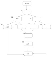
This example has a computation of "exp1" in blocks B2, B3 and B6. Assume that the remaining blocks do not effect the evaluation of "exp1".

Classic GCSE will only eliminate the computation of "exp1" found in block B3 since the evaluation in block B6 can be reached via a path which does not have an earlier computation of "exp1" (entry, B1, B7, B8, B5, B6).

PRE will eliminate the evaluations of "exp1" in blocks B3 and B6; to make the evaluation in B6 redundant, PRE will insert an evaluation of "exp1" in block B8.

While PRE is a more powerful optimization, it will tend to increase code size to improve runtime performance. Therefore, then optimizing for code size, the compiler will run the classic GCSE optimizer instead of the PRE optimizer.

Global constant/copy propagation and global common subexpression elimination are enabled by default with the -O2 optimization flag. They can also be enabled with the -fgcse flag.

sk_buff Structure

The sk_buff structure ('skb') is actually only used for storing the
metadata corresponding to a packet. The packet's data is not stored
inside the sk_buff structure itself, but in a separate buffer that is
pointed to by skb->head. The skb->end member points one byte past the
end of this data buffer.

An important design requirement for sk_buffs is being able to add data
at the end as well as at the front of the packet. As a packet travels
downwards through the network stack, each layer will usually want to
add its own header in front of the packet, and it would be nice if we
could avoid reallocating and/or copying the entire data portion of the
packet around to make more space at the front of the buffer every time
we want to do this.

To achieve this goal, the packet data is not necessarily stored at the
front of the data buffer, but some space between the front of the buffer
and the front of the packet is left unused. skb->data and skb->tail
are two extra pointers that point to the beginning and one byte past
the end of the currently used portion of the data buffer, respectively.
Both are guaranteed to point somewhere within the data buffer.
('skb->head <= skb->data <= skb->tail <= skb->end')

+----------+------------------+----------------+
| headroom | packet data | tailroom |
+----------+------------------+----------------+
skb->head skb->data skb->tail skb->end

(sorry if the figure doesnt come up well)
The function skb_headroom(skb) calculates 'skb->data - skb->head', and
indicates how many bytes we can add to the front of the packet without
having to reallocate the buffer. Similarly, skb_tailroom(skb) calculates
'skb->end - skb->tail' and indicates how many bytes we can add to the
end of the packet before having to reallocate.

Adding data to and removing data from the front of the buffer is done
with skb_push and skb_pull, respectively. These wrappers do some sanity
checks to make sure the relevant constraints on the four pointers are
maintained.

When an sk_buff is allocated by alloc_skb, skb->{head,data,tail} are all
initialised to point to the start of the data buffer. Depending on what
the skb will be used for, the caller will usually want to reserve some
headroom in anticipation of expansion of the data buffer towards the
front. This is done by calling skb_reserve().

Rough Notes on Linux Networking Stack

Table of Contents

1. Existing Optimizations
2. Packet Copies
3. ICMP Ping/Pong : Function Calls
4. Transmit Interrupts and Flow Control
5. NIC driver callbacks and ifconfig
6. Protocol Structures in the Kernel
7. skb_clone() vs. skb_copy()
8. NICs and Descriptor Rings
9. How much networking work does the ksoftirqd do?
10. Packet Requeues in Qdiscs
11. Links
12. Specific TODOs
References

1. Existing Optimizations

A great deal of thought has gone into Linux networking
implementation and many optmizations have made their way to the
kernel over the years. Some prime examples include:
* NAPI - Receive interrupts are coalesced to reduce changes of a
livelock. Thus, now each packet receive does not generate an
interrupt. Required modifications to device driver interface.
Has been in the stable kernels since 2.4.20.
* Zero-Copy TCP - Avoids the overhead of kernel-to-userspace and
userspace-to-kernel packet copying.
http://builder.com.com/5100-6372-1044112.html describes this is
some detail.

2. Packet Copies

When a packet is received, the device uses DMA to put it in main
memory (let's ignore non-DMA or non-NAPI code and drivers). An skb
is constructed by the poll() function of the device driver. After
this point, the same skb is used throughout the networking stack,
i.e., the packet is almost never copied within the kernel (it is
copied when delivered to user-space).

This design is borrowed from BSD and UNIX SVR4 - the idea is to
allocate memory for the packet only once. The packet has 4 primary
pointers - head, end, data, tail into the packet data (character
buffer). head points to the beginning of the packet - where the link
layer header starts. end points to the end of the packet. data
points to the location the current networking layer can start
reading from (i.e., it changes as the packet moves up from the link
layer, to IP, to TCP). Finally, tail is where the current protocol
layer can begin writing data to (see alloc_skb(), which sets head,
data, tail to the beginning of allocated memory block and end to
data + size).

Other implementations refer to head, end, data, tail as base, limit,
read, write respectively.

There are some instances where a packet needs to be duplicated. For
example, when running tcpdump the packet needs to be sent to the
userspace process as well as to the normal IP handler. Actually, int
this case too, a copy can be avoided since the contents of the
packet are not being modified. So instead of duplicating the packet
contents, skb_clone() is used to increase the reference count of a
packet. skb_copy() on the other hand actually duplicates the
contents of the packet and creates a completely new skb.

See also: http://oss.sgi.com/archives/netdev/2005-02/msg00125.html

A related question: When a packet is received, are the tail and end
pointers equal? Answer: NO. This is because memory for packets
received is allocated before the packet is received, and the address
and size of this memory is communicated to the NIC using receive
descriptors - so that when it is actually received the NIC can use
DMA to transfer the packet to main memory. The size allocated for a
received packet is a function of the MTU of the device. The size of
an Ethernet frame actually received could be anything less than the
MTU. Thus, tail of a received packet will point to the end of the
received data while end will point to the end of the memory
allocated for the packet.

3. ICMP Ping/Pong : Function Calls

Code path (functions called) when an ICMP ping is received (and
corresponding pong goes out), for linux 2.6.9: First the packet is
received by the NIC and it's interrupt handler will ultimately call
net_rx_action() to be called (NAPI, [1]). This will call the device
driver's poll function which will submit packets (skb's) to the
networking stack via netif_receive_skb. The rest is outlined below:
1. ip_rcv() --> ip_rcv_finish()
2. dst_input() --> skb->dst->input = ip_local_deliver()
3. ip_local_deliver() --> ip_local_deliver_finish()
4. ipprot->handler = icmp_rcv()
5. icmp_pointers[ICMP_ECHO].handler == icmp_echo() -- At this point
I guess you could say that the "receive" path is complete, the
packet has reached the top. Now the outbound (down the stack)
journey begins)
6. icmp_reply() -- Might want to look into the checks this function
does
7. icmp_push_reply()
8. ip_push_pending_frames()
9. dst_output() --> skb->dst->output = ip_output()
10. ip_output() --> ip_finish_output() --> ip_finish_output2()
11. dst->neighbour->output ==

4. Transmit Interrupts and Flow Control

Transmit interrupts are generated after every packet transmission
and this is key to flow control. However, this does have significant
performance implications under heavy transmit-related I/O (imagine a
packet forwarder where the number of transmitted packets is equal to
the number of received oned). Each device provides a means to slow
down transmit (Tx) interrupts. For example, Intel's e1000 driver
exposes "TxIntDelay" that allows transmit interrupts to be delayed
in units of 1.024 microseconds. The default value is 64, thus eavy
under heavy transmissions an interrupt's are spaced 65.536
microseconds apart. Imagine the number of transmissions that can
take place in this time.

5. NIC driver callbacks and ifconfig

Interfaces are configured using the ifconfig command. Many of these
commands will result in a function of the NIC driver being called.
For example, ifconfig eth0 up should result in the device driver's
open() function being called (open is a member of struct
net_device). ifconfig communicates with the kernel through ioctl()
on any socket. The requests are a struct ifreq (see
/usr/include/net/if.h and
http://linux.about.com/library/cmd/blcmdl7_netdevice.htm. Thus,
ifconfig eth0 up will result in the following:
1. A socket (of any kind) is opened using socket()
2. A struct ifreq is prepared with ifr_ifname set to "eth0"
3. An ioctl() with request SIOCGIFFLAGS is done to get the current
flags and then the IFF_UP and IFF_RUNNING flags are set with
another ioctl() (with request SIOCSIFFLAGS).
4. Now we're inside the kernel. sock_ioctl() is called, which in
turn calls dev_ioctl() (see net/socket.c and net/core/dev.c)
5. dev_ioctl() --> ... --> dev_open() --> driver's open()
implementation.

6. Protocol Structures in the Kernel

There are various structs in the kernel which consist of function
pointers for protocol handling. Different structures correspond to
different layers of protocols as well as whether the functions are
for synchronous handling (e.g., when recv(), send() etc. system
calls are made) or asynchronous handling (e.g., when a packet
arrives at the interface and it needs to be handled). Here is what I
have gathered about the various structures so far:
* struct packet_type - includes instantiations such as
ip_packet_type, ipv6_packet_type etc. These provide low-level,
asynchronos packet handling. When a packet arrives at the
interface, the driver ultimately submits it to the networking
stack by a call to netif_receive_skb(), which iterates to the
list of registered packet handlers and submits the skb to them.
For example, ip_packet_type.func = ip_rcv, so ip_rcv() is where
one can say the IP protocol first receives a packet that has
arrived at the interface. Packet-types are registred with the
networking stack by a call to dev_add_pack().
* struct net_proto_family - includes instantiations such as
inet_family_ops, packet_family_ops etc. Each net_proto_family
structure handles one type of address family (PF_INET etc.).
This structure is associated with a BSD socket (struct socket)
and not the networking layer representation of sockets (struct
sock). It essentially provdides a create() function which is
called in response to the socket() system call. The
implementation of create() for each family typically allocates
the struct sock and also associates other synchronous operations
(see struct proto_ops below) with the socket. To cut a long
story short - net_proto_family provides the protocol-specific
part of the socket() system call. (NOTE: Not all BSD sockets
will have a networking socket associated with it. For example,
unix sockets (the PF_UNIX address family).
unix_family_ops.create = unix_create does not allocate a struct
sock). The net_proto_family structure is registered with the
networking stack by a call to sock_register().
* struct proto_ops - includes instantiations such as
inet_stream_ops, inet_dgram_ops, packet_ops etc. These provide
implementations of networking layer synchronous calls
(connect(), bind(), recvmsg(), ioctl() etc. system calls). The
ops member of the BSD socket structure (struct socket) points to
the proto_ops associated with the socket. Unlike the above two
structures, there is no function that explicitly registers a
struct proto_ops with the networking stack. Instead, the
create() implementation of struct net_proto_family just sets the
ops field of the BSD socket to the appropriate proto_ops
structure.
* struct proto - includes instantiations such as tcp_prot,
udp_prot, raw_prot. These provide protocol handlers inside a
network family. It seems that currently this means only over-IP
protocols as I could find only the above three instantiations.
These also provide implementations for synchronous calls. The
sk_prot field of the networking socket (struct sock) points to
such a structure. The sk_prot field would get set by the create
function in struct net_proto_family and the functions provided
will be called by the implementations of functions in the struct
proto_ops structure. For example, inet_family_ops.create =
inet_create allocates a struct sock and would set sk_prot =
udp_prot in reponse to a socket(PF_INET, SOCK_DGRAM, 0); system
call. A recvfrom() system call made on the socket would then
invoke inet_dgram_ops.recvmsg = sock_common_recvmsg, which calls
sk_prot->recvmsg = udp_recvmsg. Like proto_ops, struct protos
aren't explicitly "registered" with the networking stack using a
function, but are "regsitered" by the BSD socket create()
implementation in the struct net_proto_family.
* struct net_protocol - includes instantiations such as
tcp_protocol, udp_protocol, icmp_protocol etc. These provide
asynchronous packet receive routines for IP protocols. Thus,
this structure is specific to the inet-family of protocols.
Handlers are registered using inet_add_protocol(). This
structure is used by the IP-layer routines to hand off to a
layer 4 protocol. Specifically, the IP handler (ip_rcv()) will
invoke ip_local_deliver_finish() for packets that are to be
delivered to the local host. ip_local_deliver_finish() uses a
hash table (inet_protos) to decide which function to pass the
packet to based on the protocol field in the IP header. The hash
table is populated by the call to inet_add_protocol().

7. skb_clone() vs. skb_copy()

When a packet needs to be delivered to two separate handlers (for
example, the IP layer and tcpdump), then it is "cloned" by
incrementing the reference count of the packet instead of being
"copied". Now, though the two handlers are not expected to modify
the packet contents, they can change the data pointer. So, how do we
ensure that processing by one of the handlers doesn't mess up the
data pointer for the other?

A. Umm... skb_clone means that there are separate head, tail, data,
end etc. pointers. The difference between skb_copy() and skb_clone()
is precisely this - the former copies the packet completely, while
the latter uses the same packet data but separate pointers into the
packet.

8. NICs and Descriptor Rings

NOTE: Using the Intel e1000, driver source version 5.6.10.1, as an
example. Each transmission/reception has a descriptor - a "handle"
used to access buffer data somewhat like a file descriptor is a
handle to access file data. The descriptor format would be NIC
dependent as the hardware understands and reads/writes to the
descriptor. The NIC maintains a circular ring of descriptors, i.e.,
the number of descriptors for TX and RX is fixed (TxDescriptors,
RxDescriptors module parameters for the e1000 kernel module) and the
descriptors are used like a circular queue.

Thus, there are three structures:
* Descriptor Ring (struct e1000_desc_ring) - The list of
descriptors. So, ring[0], ring[1] etc. are individual
descriptors. The ring is typically allocated just once and thus
the DMA mapping of the ring is "consistent". Each descriptor in
the ring will thus have a fixed DMA and memory address. In the
e1000, the device registers TDBAL, TDBAH, TDLEN stand for
"Transmit Descriptors Base Address Low", "High" and "Length" (in
bytes of all descriptors). Similarly, there are RDBAL, RDBAH,
RDLEN
* Descriptors (struct e1000_rx_desc and struct e1000_tx_desc) -
Essentially, this stores the DMA address of the buffer which
contains actual packet data, plus some other accounting
information such as the status (transmission successsful?
receive complete? etc.), errors etc.
* Buffers - Now actual data cannot have a "consistent" DMA
mapping, meaning we cannot ensure that all skbuffs for a
particular device always have some specific memory addresses
(those that have been setup for DMA). Instead, "streaming" DMA
mappings need to be used. Each descriptor thus contains the DMA
address of a buffer that has been setup for streaming mapping.
The hardware uses that DMA address to pickup a packet to be sent
or to place a received packet. Once the kernel's stack picks up
the buffer, it can allocate new resources (a new buffer) and
tell the NIC to use that buffer next time by setting up a new
streaming mapping and putting the new DMA handle in the
descriptor.
The e1000 uses a struct e1000_buffer as a wrapper around the
actual buffer. The DMA mapping however is setup only for
skb->data, i.e., where raw packet data is to be placed.

9. How much networking work does the ksoftirqd do?

Consider what the NET_RX_SOFTIRQ does:
1. Each softirq invokation (do_softirq()) processes up to
net.core.netdev_max_backlog x MAX_SOFTIRQ_RESTART packets, if
available. The default values lead to 300 x 10 = 3000 pkts.
2. Every interrupt calls do_softirq() when exitting (irq_exit()) -
including the timer interrupt and NMIs too?
3. Default transmit/receive ring sizes on the NIC are less than
3000 (the e1000 for example defaults to 256 and can have at most
4096 descriptors on its ring)

Thus, the number of times ksoftirqd will be switched in/out depends
on how much processing is done by do_softirq() invokations on
irq_exit(). If the softirq handling on interrupt is able to clean up
the NIC ring faster than a new packet comes in, then ksoftirqd won't
be doing anything. Specifically, if the inter-packet-gap is greater
than the time it takes to pick-up and process a single packet from
the NIC, then ksoftirq will not be scheduled (and if the number of
descriptors on the NIC is less than 3000).

Without going into details, some quick experimental verification:
Machine A continuously generates UDP packets for Machine B which is
running an "sink" application, i.e., it just loops on a recvfrom().
When the size of the packet sent from A was 60 bytes (and
inter-packet gap averaged 1.5µs), then the ksoftirqd thread on B
observed a total of 375 context swithces (374 involuntary and 1
voluntary). When the packet size was 1280 bytes (and now
inter-packet gap increased almost 7 times to 10µs) then the
ksoftirqd thread was NEVER scheduled (0 context switches). The
single voluntary context switch in the former case probably happened
after all packets were processed (i.e., the sender stopped sending
and the receiver processed all that it got).

10. Packet Requeues in Qdiscs

The queueing discipline (struct Qdisc) provides a requeue().
Typically, packets are dequeued from the qdisc and submitted to the
device driver (the hard_start_xmit function in struct net_device).
However, at times it is possible that the device driver is "busy",
so the dequeued packet must be "requeued". "Busy" here means that
the xmit_lock of the device was held. It seems that this lock is
acquired at two places: (1) qdisc_restart() and (2) dev_watchdog().
The former handles packet dequeueing from the qdisc, acquiring the
xmit_lock and then submitting the packet to the device driver
(hard_start_xmit()) or alternatively requeuing the packet if the
xmit_lock was already held by someone else. The latter is invoked
asynchronously, periodically - its part of the watchdog timer
mechanism.

My understanding is that two threads cannot be in qdisc_restart()
for the same qdisc at the same time, however the xmit_lock may have
been acquired by the watchdog timer function causing a requeue.

11. Links

This is just a dump of links that might be useful.
* http://www.spec.org and SpecWeb http://www.spec.org/web99/
* linux-net and netdev mailing lists:
http://www.ussg.iu.edu/hypermail/linux/net/ and
http://oss.sgi.com/projects/netdev/archive/
* Linux Traffic Control HOWTO

12. Specific TODOs

* Study watchdog timer mechanism and figure out how flow control
is implemented in the receive and transmit side

References

[3] Beyond Softnet. Jamal Hadi Salim, Robert Olsson, and Alexey
Kuznetsov. Nov 2001. USENIX. 5. .

[5] A Map of the Networking Code in Linux Kernel 2.4.20. Miguel Rio,
Mathieu Goutelle, Tom Kelly, Richard Hugh-Jones, Jean-Phillippe
Martin-Flatin, and Yee-Ting Li. Mar 2004.

[4] Understanding the Linux Kernel. Daniel P. Bovet and Marco
Cesati. O'Reilly & Associates. 2nd Edition. 81-7366-589-3.

volatile

The use of volatile is poorly understood by many programmers. This is not surprising, as most C texts dismiss it in a sentence or two.

Have you experienced any of the following in your C/C++ embedded code?

* Code that works fine-until you turn optimization on
* Code that works fine-as long as interrupts are disabled
* Flaky hardware drivers
* Tasks that work fine in isolation-yet crash when another task is enabled

If you answered yes to any of the above, it's likely that you didn't use the C keyword volatile. You aren't alone. The use of volatile is poorly understood by many programmers. This is not surprising, as most C texts dismiss it in a sentence or two.

volatile is a qualifier that is applied to a variable when it is declared. It tells the compiler that the value of the variable may change at any time-without any action being taken by the code the compiler finds nearby. The implications of this are quite serious. However, before we examine them, let's take a look at the syntax.

Syntax

To declare a variable volatile, include the keyword volatile before or after the data type in the variable definition. For instance both of these declarations will declare foo to be a volatile integer:

volatile int foo;
int volatile foo;

Now, it turns out that pointers to volatile variables are very common. Both of these declarations declare foo to be a pointer to a volatile integer:

volatile int * foo;
int volatile * foo;

Volatile pointers to non-volatile variables are very rare (I think I've used them once), but I'd better go ahead and give you the syntax:

int * volatile foo;

And just for completeness, if you really must have a volatile pointer to a volatile variable, then:

int volatile * volatile foo;

Incidentally, for a great explanation of why you have a choice of where to place volatile and why you should place it after the data type (for example, int volatile * foo), consult Dan Sak's column, "Top-Level cv-Qualifiers in Function Parameters" (February 2000, p. 63).

Finally, if you apply volatile to a struct or union, the entire contents of the struct/union are volatile. If you don't want this behavior, you can apply the volatile qualifier to the individual members of the struct/union.

Use

A variable should be declared volatile whenever its value could change unexpectedly. In practice, only three types of variables could change:

* Memory-mapped peripheral registers
* Global variables modified by an interrupt service routine
* Global variables within a multi-threaded application

Peripheral registers

Embedded systems contain real hardware, usually with sophisticated peripherals. These peripherals contain registers whose values may change asynchronously to the program flow. As a very simple example, consider an 8-bit status register at address 0x1234. It is required that you poll the status register until it becomes non-zero. The nave and incorrect implementation is as follows:

UINT1 * ptr = (UINT1 *) 0x1234;

// Wait for register to become non-zero.
while (*ptr == 0);
// Do something else.

This will almost certainly fail as soon as you turn the optimizer on, since the compiler will generate assembly language that looks something like this:

mov ptr, #0x1234 mov a, @ptr loop bz loop

The rationale of the optimizer is quite simple: having already read the variable's value into the accumulator (on the second line), there is no need to reread it, since the value will always be the same. Thus, in the third line, we end up with an infinite loop. To force the compiler to do what we want, we modify the declaration to:

UINT1 volatile * ptr =
(UINT1 volatile *) 0x1234;

The assembly language now looks like this:

mov ptr, #0x1234
loop mov a, @ptr
bz loop

The desired behavior is achieved.

Subtler problems tend to arise with registers that have special properties. For instance, a lot of peripherals contain registers that are cleared simply by reading them. Extra (or fewer) reads than you are intending can cause quite unexpected results in these cases.

Interrupt service routines

Interrupt service routines often set variables that are tested in main line code. For example, a serial port interrupt may test each received character to see if it is an ETX character (presumably signifying the end of a message). If the character is an ETX, the ISR might set a global flag. An incorrect implementation of this might be:

int etx_rcvd = FALSE;

void main()
{
...
while (!ext_rcvd)
{
// Wait
}
...
}

interrupt void rx_isr(void)
{
...
if (ETX == rx_char)
{
etx_rcvd = TRUE;
}
...
}

With optimization turned off, this code might work. However, any half decent optimizer will "break" the code. The problem is that the compiler has no idea that etx_rcvd can be changed within an ISR. As far as the compiler is concerned, the expression !ext_rcvd is always true, and, therefore, you can never exit the while loop. Consequently, all the code after the while loop may simply be removed by the optimizer. If you are lucky, your compiler will warn you about this. If you are unlucky (or you haven't yet learned to take compiler warnings seriously), your code will fail miserably. Naturally, the blame will be placed on a "lousy optimizer."

The solution is to declare the variable etx_rcvd to be volatile. Then all of your problems (well, some of them anyway) will disappear.

Multi-threaded applications

Despite the presence of queues, pipes, and other scheduler-aware communications mechanisms in real-time operating systems, it is still fairly common for two tasks to exchange information via a shared memory location (that is, a global). When you add a pre-emptive scheduler to your code, your compiler still has no idea what a context switch is or when one might occur. Thus, another task modifying a shared global is conceptually identical to the problem of interrupt service routines discussed previously. So all shared global variables should be declared volatile. For example:

int cntr;

void task1(void)
{
cntr = 0;
while (cntr == 0)
{
sleep(1);
}
...
}

void task2(void)
{
...
cntr++;
sleep(10);
...
}

This code will likely fail once the compiler's optimizer is enabled. Declaring cntr to be volatile is the proper way to solve the problem.

Final thoughts

Some compilers allow you to implicitly declare all variables as volatile. Resist this temptation, since it is essentially a substitute for thought. It also leads to potentially less efficient code.

Also, resist the temptation to blame the optimizer or turn it off. Modern optimizers are so good that I cannot remember the last time I came across an optimization bug. In contrast, I come across failures to use volatile with depressing frequency.

If you are given a piece of flaky code to "fix," perform a grep for volatile. If grep comes up empty, the examples given here are probably good places to start looking for problems.

Configuration options on 2.6.x kernels

On the 2.6.x kernels there are four main frontend programs: config, menuconfig, and xconfig.

config is the least user-friendly option as it merely presents a series of questions that must be answered sequentially. Alas, if an error is made you must begin the process from the top. Pressing Enter will accept the default entry which is in upper case.

oldconfig will read the defaults from an existing .config and rewrite necessary links and files. Use this option if you've made minor changes to source files or need to script the rebuild process.

menuconfig is an ncurses based frontend. Your system must have the ncurses-devel libraries installed in order to use this utility. As the help text at the top of the screen indicates, use the arrow keys to navigate the menu. Press Enter to select sub-menus. Press the highlighted letter on each option to jump directly to that option. To build an option directly into the kernel, press Y. To disable an option entirely, press N. To build an option as a loadable module, press M. You can also access content-specific help screens by pressing ? on each page or selecting HELP from the lower menu. Figure 1 in the Section called Configuring the 2.4.x kernels shows an example screen from the 2.4.x kernel series.

xconfig is a graphical frontend using qconf by Roman Zippel. It requires the qt and X libraries to build and use. The interface is intuitive and customizable. Online help is automatically shown for each kernel configuration option. It also can show dependency information for each module which can help diagnose build errors. Figure 3 shows an example of the xconfig screen. From the online help:


For each option, a blank box indicates the feature is disabled, a check
indicates it is enabled, and a dot indicates that it is to be compiled
as a module. Clicking on the box will cycle through the three states.
If you do not see an option (e.g., a device driver) that you believe
should be present, try turning on Show All Options under the Options menu.
Although there is no cross reference yet to help you figure out what other
options must be enabled to support the option you are interested in, you can
still view the help of a grayed-out option.

--qconf help

Figure 3. make xconfig

Once you have decided which configuration option to use, start the process with make followed by either config, menuconfig, or xconfig. For example:

$ make menuconfig


The system will take a few moments to build the configuration utility. Next you will be presented with the configuration menus. Though similar to the 2.4.x series, the 2.6.x menu is more logically organized with better grouping of sub-modules. Following are some of the top level configuration options in the 2.6 kernel.

Code Maturity Level Options

This option allows configuration of alpha-quality software or obsoleted drivers. It is best to disable this option if the kernel is intended for a stable production system. If you require an experimental feature in the kernel, such as a driver for new hardware, then enable this option but be aware that it "may not meet the normal level of reliability" as more rigorously tested code.
General Setup

This section contains options for sysctl support, a feature allowing run-time configuration of the kernel. A new feature, kernel .config support, allows the complete kernel configuration to be viewed during run-time. This addresses many requests to be able to see what features were compiled into the kernel.
Loadable Module Support

You will almost certainly want to enable module support. If you will need third-party kernel modules you will also need to enable Set Version Information on All Module Symbols.
Processor Type and Features

This is perhaps the most important configuration choice. we determin our processor type by examining /proc/cpuinfo and we use that information here to select the appropriate processor. Included in this submenu are features such as Preemptible Kernel which can improve desktop responsiveness, Symmetric Multi-processing Support for machines with multiple CPUs, and High Memory Support for machines with more than 1G of RAM.
Power Management Options

Found here are options for ACPI and CPU Frequency Scaling which can dramatically improve laptop power usage. Read the Documentation/power file for more information.
Bus Options ( PCI, PCMCIA, EISA, MCA, ISA)

Here are found options for all system bus devices. On modern machines the ISA and MCA support can often be disabled.
Executable File Formats

Interesting features here include the kernel support for miscellaneous binaries, which can allow seamless operation of non-Linux binaries with a little userland help.
Device Drivers

All the device-driver configuration options that were previously scattered throughout the 2.4.x menus are now neatly organized under this option. Features such as SCSI support, graphic card optimizations, sound, USB and other hardware are configured here.
File Systems

Found here are options for filesystems which are supported by the kernel, such as EXT2 and ReiserFS. It is best to build support for the root filesystems directly into the kernel rather than as a module.
Security Options

Interesting options here include support for NSA Security Enhanced Linux and other, somewhat experimental, features to increase security.

Dynamic Kernels: Modularized Device Drivers

Although this is very old article, gives u lot of knowledge about the device drivers.
Some of the things mentioned here changed by this day.

By Alessandro Rubini on Fri, 1996-03-01 02:00. SysAdmin
This is the first in a series of four articles co-authored by Alessandro Rubini and Georg Zezchwitz which present a practical approach to writing Linux device drivers as kernel loadable modules. This installment presents and introduction to thte topic, preparing the reader to understand next month's installment.
Kernel modules are a great feature of recent Linux kernels. Although most users feel modules are only a way to free some memory by keeping the floppy driver out of the kernel most of the time, the real benefit of using modules is support for adding additional devices without patching the kernel source. In the next few Kernel Korners Georg Zezschwitz and I will try to introduce the ``art'' of writing a powerful module---while avoiding common design errors.
What is a device?
A device driver is the lowest level of the software that runs on a computer, as it is directly bound to the hardware features of the device.
The concept of ``device driver'' is quite abstract, actually, and the kernel can be considered like it was a big device driver for a device called ``computer''. Usually, however, you don't consider your computer a monolithic entity, but rather a CPU equipped with peripherals. The kernel can thus be considered as an application running on top of the device drivers: each driver manages a single part of the computer, while the kernel-proper builds process scheduling and file-system access on top of the available devices.
See Figure 1.
A few mandatory drivers are ``hardwired'' in the kernel, such as the processor driver and the the memory driver; the others are optional, and the computer is usable both with and without them---although a kernel with neither the console driver nor the network driver is pointless for a conventional user.
The description above is somehow a simplistic one, and slightly philosophical too. Real drivers interact in a complex way and a clean distinction among them is sometimes difficult to achieve.
In the Unix world things like the network driver and a few other complex drivers belong to the kernel, and the name of device driver is reserved to the low-level software interface to devices belonging to the following three groups:
character devices
Those which can be considered files, in that they can be read-from and/or written-to. The console (i.e. monitor and keyboard) and the serial/parallel ports are examples of character devices. Files like /dev/tty0 and /dev/cua0 provide user access to the device. A char device usually can only be accessed sequentially.
block devices
Historically: devices which can be read and written only in multiples of the block-size, often 512 or 1024 bytes. These are devices on which you can mount a filesystem, most notably disks. Files like /dev/hda1 provide access to the devices. Blocks of block devices are cached by the buffer cache. Unix provides uncached character devices corresponding to block devices, but Linux does not.
network interfaces
Network interfaces don't fall in the device-file abstraction. Network interfaces are identified by means of a name (such as eth0 or plip1) but they are not mapped to the filesystem. It would be theoretically possible, but it is impractical from a programming and performance standpoint; a network interface can only transfer packets, and the file abstraction does not efficiently manage structured data like packets.

The description above is rather sketchy, and each flavour of Unix differs in some details about what is a block device. It doesn't make too much a difference, actually, because the distinction is only relevant inside the kernel, and we aren't going to talk about block drivers in detail.
What is missing in the previous representation is that the kernel also acts as a library for device drivers; drivers request services from the kernel. Your module will be able to call functions to perform memory allocation, filesystem access, and so on.
As far as loadable modules are concerned, any of the three driver-types can be constructed as a module. You can also build modules to implement filesystems, but this is outside of our scope.
These columns will concentrate on character device drivers, because special (or home-built) hardware fits the character device abstraction most of the time. There are only a few differences between the three types, and so to avoid confusion, we'll only cover the most common type.
You can find an introduction to block drivers in issues 9, 10, and 11 of Linux Journal, as well as in the Linux Kernel Hackers' Guide. Although both are slightly outdated, taken together with these columns, they should give you enough information to get started.
What is a module?
A module is a code segment which registers itself with the kernel as a device driver, is called by the kernel in order to communicate with the device, and in turn invokes other kernel functions to accomplish its tasks. Modules utilize a clean interface between the ``kernel proper'' and the device, which both makes the modules easy to write and keeps the kernel source code from being cluttered.
The module must be compiled to object code (no linking; leave the compiled code in .o files), and then loaded into the running kernel with insmod. The insmod program is a runtime linker, which resolves any undefined symbols in the module to addresses in the running kernel by means of the kernel symbol table.
This means that you can write a module much like a conventional C-language program, and you can call functions you don't define, in the same way you usually call printf() and fopen() in your application. However, you can count only on a minimal set of external functions, which are the public functions provided by the kernel. insmod will put the right kernel-space addresses in your compiled module wherever your code calls a kernel function, then insert the module into the running Linux kernel.
If you are in doubt whether a kernel-function is public or not, you can look for its name either in the source file /usr/src/linux/kernel/ksyms.c or in the run-time table /proc/ksyms.
To use make to compile your module, you'll need a Makefile as simple as the following one:

TARGET = myname

ifdef DEBUG
# -O is needed, because of "extern inline"
# Add -g if your gdp is patched and can use it
CFLAGS = -O -DDEBUG_$(TARGET) -D__KERNEL__ -Wall
else
CFLAGS = -O3 -D__KERNEL__ -fomit-frame-pointer
endif

all: $(TARGET).o

As you see, no special rule is needed to build a module, only the correct value for CFLAGS. I recommend that you include debugging support in your code, because without patches, gdb isn't able to take advantage of the symbol information provided by the -g flag to a module while it is part of the running kernel.
Debugging support will usually mean extra code to print messages from within the driver. Using printk() for debugging is powerful, and the alternatives are running a debugger on the kernel, peeking in /dev/mem, and other extremely low-level techniques. There are a few tools available on the Internet to help use these other techniques, but you need to be conversant with gdb and be able to read real kernel code in order to benefit from them. The most interesting tool at time of writing is kdebug-1.1, which lets you use gdb on a running kernel, examining or even changing kernel data structures (including those in loaded kernel modules) while the kernel is running. Kdebug is available for ftp from sunsite.unc.edu and its mirrors under /pub/Linux/kernel.
Just to make things a little harder, the kernel equivalent of the standard printf() function is called printk(), because it does not work exactly the same as printf(). Before 1.3.37, conventional printk()'s generated lines in /var/adm/messages, while later kernels will dump them to the console. If you want quiet logging (only within the messages file, via syslogd) you must prepend the symbol KERN_DEBUG to the format string. KERN_DEBUG and similar symbols are simply strings, which get concatenated to your format string by the compiler. This means that you must not put a comma between KERN_DEBUG and the format string. These symbols can be found in , and are documented there. Also, printk() does not support floating point formats.
Remember, that syslog write to the messages file as soon as possible, in order to save all messages on disk in case of a system crash. This means that an over-printk-ed module will slow down perceptibly, and will fill your disk in a short time.
Almost any module misbehaviour will generate an [cw]Oops[ecw] message from the kernel. An Oops is what happens when the kernel gets an exception from kernel code. In other words, Oopses are the equivalent of segmentation faults in user space, though no core file is generated. The result is usually the sudden destruction of the responsible process, and a few lines of low-level information in the messages file. Most Oops messages are the result of dereferencing a NULL pointer.
This way to handle disasters is a friendly one, and you'll enjoy it whenever your code is faulty: most other Unices produce a kernel panic instead. This does not mean that Linux never panics. You must be prepared to generate panics whenever you write functions that operate outside of a process context, such as within interrupt handlers and timer callbacks.
The scarce, nearly unintelligible information included with the [cw]Oops[ecw] message represents the processor state when the code faulted, and can be used to understand where the error is. A tool called ksymoops is able to print more readable information out of the oops, provided you have a kernel map handy. The map is what is left in /usr/src/linux/System.map after a kernel compilation. Ksymoops was distributed within util-linux-2.4, but was removed in 2.5 because it has been included in the kernel distribution during the linux-1.3 development.
If you really understand the Oops message, you can use it as you want, like invoking gdb off-line to disassemble the whole responsible function. if you understand neither the Oops nor the ksymoops output, you'd better add some more debugging printk() code, recompile, and reproduce the bug.
The following code can ease management of debugging messages. It must reside in the module's public include file, and will work for both kernel code (the module) and user code (applications). Note however that this code is gcc-specific. Not too big a problem for a kernel module, which is gcc-dependent anyway. This code was suggested by Linus Torvalds, as an enhancement over my previous ansi-compliant approach.
#ifndef PDEBUG
# ifdef DEBUG_modulename
# ifdef __KERNEL__
# define PDEBUG(fmt, args...) printk (KERN_DEBUG fmt , ## args)
# else
# define PDEBUG(fmt, args...) fprintf (stderr, fmt , ## args)
# endif
# else
# define PDEBUG(fmt, args...)
# endif
#endif

#ifndef PDEBUGG
# define PDEBUGG(fmt, args...)
#endif

After this code, every PDEBUG("any %i or %s...\n", i, s); in the module will result in a printed message only if the code is compiled with -DDEBUG_modulename, while PDEBUGG() with the same arguments will expand to nothing. In user mode applications, it works the same, except that the message is printed to stderr instead of the messages file.
Using this code, you can enable or disable any message by removing or adding a single G character.
Writing Code
Let's look at what kind of code must go inside the module. The simple answer is ``whatever you need''. In practice, you must remember that the module is kernel code, and must fit a well-defined interface with the rest of Linux.
Usually, you start with header inclusion. And you begin to have contraints: you must always define the __KERNEL__ symbol before including any header unless it is defined in your makefile, and you must only include files pertaining to the and hierarchies. Sure, you can include your module-specific header, but never, ever, include library specific files, such as or .
The code fragment in Listing 1 represents the first lines of source of a typical character driver. If you are going to write a module, it will be easier to cut and paste these lines from existing source rather than copying them by hand from this article.
#define __KERNEL__ /* kernel code */

#define MODULE /* always as a module */
#include /* can't do without it */
#include /* and this too */

/*
* Then include whatever header you need.
* Most likely you need the following:
*/
#include /* ulong and friends */
#include /* current, task_struct, other goodies */
#include /* O_NONBLOCK etc. */
#include /* return values */
#include /* request_region() */
#include /* system name and global items */
#include /* kmalloc, kfree */

#include /* inb() inw() outb() ... */
#include /* unreadable, but useful */

#include "modulename.h" /* your own material */

After including the headers, there comes actual code. Before talking about specific driver functionality---most of the code---it is worth noting that there exist two module-specific functions, which must be defined in order for the module to be loaded:
int init_module (void);
void cleanup_module (void);

The first is in charge of module initialization (looking for the related hardware and registering the driver in the appropriate kernel tables), while the second is in charge of releasing any resources the module has allocated and deregistering the driver from the kernel tables.
If these functions are not there, insmod will fail to load your module.
The init_module() function returns 0 on success and a negative value on failure. The cleanup_module() function returns void, because it only gets invoked when the module is known to be unloadable. A kernel module keeps a usage count, and cleanup_module() is only called when that counter's value is 0 (more on this later on).
Skeletal code for these two functions will be presented in the next installment. Their design is fundamental for proper loading and unloading of the module, and a few details must dealt with. So here, I'll introduce you to each of the details, so that next month I can present the structure without explaining all the details.

contd....

Hardware and Software IRQs

Hardware Interrupts (Hard IRQs)

Timer ticks, network cards and keyboard are examples of real hardware which produce interrupts at any time. The kernel runs interrupt handlers, which services the hardware. The kernel guarantees that this handler is never re-entered: if another interrupt arrives, it is queued (or dropped). Because it disables interrupts, this handler has to be fast: frequently it simply acknowledges the interrupt, marks a `software interrupt' for execution and exits.
You can tell you are in a hardware interrupt, because in_irq() returns true.


Software Interrupt Context: Bottom Halves, Tasklets, softirqs

Whenever a system call is about to return to userspace, or a hardware interrupt handler exits, any `software interrupts' which are marked pending (usually by hardware interrupts) are run (kernel/softirq.c).
Much of the real interrupt handling work is done here. Early in the transition to SMP, there were only `bottom halves' (BHs), which didn't take advantage of multiple CPUs. Shortly after we switched from wind-up computers made of match-sticks and snot, we abandoned this limitation.
include/linux/interrupt.h lists the different BH's. No matter how many CPUs you have, no two BHs will run at the same time. This made the transition to SMP simpler, but sucks hard for scalable performance. A very important bottom half is the timer BH (include/linux/timer.h): you can register to have it call functions for you in a given length of time.
2.3.43 introduced softirqs, and re-implemented the (now deprecated) BHs underneath them. Softirqs are fully-SMP versions of BHs: they can run on as many CPUs at once as required. This means they need to deal with any races in shared data using their own locks. A bitmask is used to keep track of which are enabled, so the 32 available softirqs should not be used up lightly. (Yes, people will notice).
tasklets (include/linux/interrupt.h) are like softirqs, except they are dynamically-registrable (meaning you can have as many as you want), and they also guarantee that any tasklet will only run on one CPU at any time, although different tasklets can run simultaneously (unlike different BHs).
You can tell you are in a softirq (or bottom half, or tasklet) using the in_softirq() macro (include/asm/softirq.h).

GCC Optimization

Here's what the O options mean in GCC, why some optimizations aren't optimal after all and how you can make specialized optimization choices for your application.

In this article, we explore the optimization levels provided by the GCC compiler toolchain, including the specific optimizations provided in each. We also identify optimizations that require explicit specifications, including some with architecture dependencies. This discussion focuses on the 3.2.2 version of gcc (released February 2003), but it also applies to the current release, 3.3.2.

Levels of Optimization

Let's first look at how GCC categorizes optimizations and how a developer can control which are used and, sometimes more important, which are not. A large variety of optimizations are provided by GCC. Most are categorized into one of three levels, but some are provided at multiple levels. Some optimizations reduce the size of the resulting machine code, while others try to create code that is faster, potentially increasing its size. For completeness, the default optimization level is zero, which provides no optimization at all. This can be explicitly specified with option -O or -O0.
Level 1 (-O1)

The purpose of the first level of optimization is to produce an optimized image in a short amount of time. These optimizations typically don't require significant amounts of compile time to complete. Level 1 also has two sometimes conflicting goals. These goals are to reduce the size of the compiled code while increasing its performance. The set of optimizations provided in -O1 support these goals, in most cases. These are shown in Table 1 in the column labeled -O1. The first level of optimization is enabled as:

gcc -O1 -o test test.c



Table 1. GCC optimizations and the levels at which they are enabled.

Any optimization can be enabled outside of any level simply by specifying its name with the -f prefix, as:

gcc -fdefer-pop -o test test.c



We also could enable level 1 optimization and then disable any particular optimization using the -fno- prefix, like this:

gcc -O1 -fno-defer-pop -o test test.c



This command would enable the first level of optimization and then specifically disable the defer-pop optimization.
Level 2 (-O2)

The second level of optimization performs all other supported optimizations within the given architecture that do not involve a space-speed trade-off, a balance between the two objectives. For example, loop unrolling and function inlining, which have the effect of increasing code size while also potentially making the code faster, are not performed. The second level is enabled as:

gcc -O2 -o test test.c



Table 1 shows the level -O2 optimizations. The level -O2 optimizations include all of the -O1 optimizations, plus a large number of others.
Level 2.5 (-Os)

The special optimization level (-Os or size) enables all -O2 optimizations that do not increase code size; it puts the emphasis on size over speed. This includes all second-level optimizations, except for the alignment optimizations. The alignment optimizations skip space to align functions, loops, jumps and labels to an address that is a multiple of a power of two, in an architecture-dependent manner. Skipping to these boundaries can increase performance as well as the size of the resulting code and data spaces; therefore, these particular optimizations are disabled. The size optimization level is enabled as:

gcc -Os -o test test.c



In gcc 3.2.2, reorder-blocks is enabled at -Os, but in gcc 3.3.2 reorder-blocks is disabled.
Level 3 (-O3)

The third and highest level enables even more optimizations (Table 1) by putting emphasis on speed over size. This includes optimizations enabled at -O2 and rename-register. The optimization inline-functions also is enabled here, which can increase performance but also can drastically increase the size of the object, depending upon the functions that are inlined. The third level is enabled as:

gcc -O3 -o test test.c



Although -O3 can produce fast code, the increase in the size of the image can have adverse effects on its speed. For example, if the size of the image exceeds the size of the available instruction cache, severe performance penalties can be observed. Therefore, it may be better simply to compile at -O2 to increase the chances that the image fits in the instruction cache.
Architecture Specification

The optimizations discussed thus far can yield significant improvements in software performance and object size, but specifying the target architecture also can yield meaningful benefits. The -march option of gcc allows the CPU type to be specified (Table 2).

Table 2. x86 Architectures
Target CPU Types -march= Type
i386 DX/SX/CX/EX/SL i386
i486 DX/SX/DX2/SL/SX2/DX4 i486
487 i486
Pentium pentium
Pentium MMX pentium-mmx
Pentium Pro pentiumpro
Pentium II pentium2
Celeron pentium2
Pentium III pentium3
Pentium 4 pentium4
Via C3 c3
Winchip 2 winchip2
Winchip C6-2 winchip-c6
AMD K5 i586
AMD K6 k6
AMD K6 II k6-2
AMD K6 III k6-3
AMD Athlon athlon
AMD Athlon 4 athlon
AMD Athlon XP/MP athlon
AMD Duron athlon
AMD Tbird athlon-tbird

The default architecture is i386. GCC runs on all other i386/x86 architectures, but it can result in degraded performance on more recent processors. If you're concerned about portability of an image, you should compile it with the default. If you're more interested in performance, pick the architecture that matches your own.

Let's now look at an example of how performance can be improved by focusing on the actual target. Let's build a simple test application that performs a bubble sort over 10,000 elements. The elements in the array have been reversed to force the worst-case scenario. The build and timing process is shown in Listing 1.

Listing 1. Effects of Architecture Specification on a Simple Application


[mtj@camus]$ gcc -o sort sort.c -O2
[mtj@camus]$ time ./sort
real 0m1.036s
user 0m1.030s
sys 0m0.000s
[mtj@camus]$ gcc -o sort sort.c -O2 -march=pentium2
[mtj@camus]$ time ./sort
real 0m0.799s
user 0m0.790s
sys 0m0.010s
[mtj@camus]$

By specifying the architecture, in this case a 633MHz Celeron, the compiler can generate instructions for the particular target as well as enable other optimizations available only to that target. As shown in Listing 1, by specifying the architecture we see a time benefit of 237ms (23% improvement).

Although Listing 1 shows an improvement in speed, the drawback is that the image is slightly larger. Using the size command (Listing 2), we can identify the sizes of the various sections of the image.

Listing 2. Size Change of the Application from Listing 1


[mtj@camus]$ gcc -o sort sort.c -O2
[mtj@camus]$ size sort
text data bss dec hex filename
842 252 4 1098 44a sort
[mtj@camus]$ gcc -o sort sort.c -O2 -march=pentium2
[mtj@camus]$ size sort
text data bss dec hex filename
870 252 4 1126 466 sort
[mtj@camus]$

From Listing 2, we can see that the instruction size (text section) of the image increased by 28 bytes. But in this example, it's a small price to pay for the speed benefit.
Math Unit Optimizations

Some specialized optimizations require explicit definition by the developer. These optimizations are specific to the i386 and x86 architectures. A math unit, for one, can be specified, although in many cases it is automatically defined based on the specification of a target architecture. Possible units for the -mfpmath= option are shown in Table 3.

Table 3. Math Unit Optimizations
Option Description
387 Standard 387 Floating Point Coprocessor
sse Streaming SIMD Extensions (Pentium III, Athlon 4/XP/MP)
sse2 Streaming SIMD Extensions II (Pentium 4)

The default choice is -mfpmath=387. An experimental option is to specify both sse and 387 (-mfpmath=sse,387), which attempts to use both units.
Alignment Optimizations

In the second optimization level, we saw that a number of alignment optimizations were introduced that had the effect of increasing performance but also increasing the size of the resulting image. Three additional alignment optimizations specific to this architecture are available. The -malign-int option allows types to be aligned on 32-bit boundaries. If you're running on a 16-bit aligned target, -mno-align-int can be used. The -malign-double controls whether doubles, long doubles and long-longs are aligned on two-word boundaries (disabled with -mno-align-double). Aligning doubles provides better performance on Pentium architectures at the expense of additional memory.

Stacks also can be aligned by using the option -mpreferred-stack-boundary. The developer specifies a power of two for alignment. For example, if the developer specified -mpreferred-stack-boundary=4, the stack would be aligned on a 16-byte boundary (the default). On the Pentium and Pentium Pro targets, stack doubles should be aligned on 8-byte boundaries, but the Pentium III performs better with 16-byte alignment.
Speed Optimizations

For applications that utilize standard functions, such as memset, memcpy or strlen, the -minline-all-stringops option can increase performance by inlining string operations. This has the side effect of increasing the size of the image.

Loop unrolling occurs in the process of minimizing the number of loops by doing more work per iteration. This process increases the size of the image, but it also can increase its performance. This option can be enabled using the -funroll-loops option. For cases in which it's difficult to understand the number of loop iterations, a prerequisite for -funroll-loops, all loops can be unrolled using the -funroll-all-loops optimization.

A useful option that has the disadvantage of making an image difficult to debug is -momit-leaf-frame-pointer. This option keeps the frame pointer out of a register, which means less setup and restore of this value. In addition, it makes the register available for the code to use. The optimization -fomit-frame-pointer also can be useful.

When operating at level -O3 or having -finline-functions specified, the size limit of the functions that may be inlined can be specified through a special parameter interface. The following command illustrates capping the size of the functions to inline at 40 instructions:

gcc -o sort sort.c --param max-inline-insns=40



This can be useful to control the size by which an image is increased using -finline-functions.
Code Size Optimizations

The default stack alignment is 4, or 16 words. For space-constrained systems, the default can be minimized to 8 bytes by using the option -mpreferred-stack-boundary=2. When constants are defined, such as strings or floating-point values, these independent values commonly occupy unique locations in memory. Rather than allow each to be unique, identical constants can be merged together to reduce the space that's required to hold them. This particular optimization can be enabled with -fmerge-constants.
Graphics Hardware Optimizations

Depending on the specified target architecture, certain other extensions are enabled. These also can be enabled or disabled explicitly. Options such as -mmmx and -m3dnow are enabled automatically for architectures that support them.
Other Possibilities

We've discussed many optimizations and compiler options that can increase performance or decrease size. Let's now look at some fringe optimizations that may provide a benefit to your application.

The -ffast-math optimization provides transformations likely to result in correct code but it may not adhere strictly to the IEEE standard. Use it, but test carefully.

When global common sub-expression elimination is enabled (-fgcse, level -O2 and above), two other options may be used to minimize load and store motions. Optimizations -fgcse-lm and -fgcse-sm can migrate loads and stores outside of loops to reduce the number of instructions executed within the loop, therefore increasing the performance of the loop. Both -fgcse-lm (load-motion) and -fgcse-sm (store-motion) should be specified together.

The -fforce-addr optimization forces the compiler to move addresses into registers before performing any arithmetic on them. This is similar to the -fforce-mem option, which is enabled automatically in optimization levels -O2, -Os and -O3.

A final fringe optimization is -fsched-spec-load, which works with the -fschedule-insns optimization, enabled at -O2 and above. This optimization permits the speculative motion of some load instructions to minimize execution stalls due to data dependencies.